


Network Traffic
Visualize network traffic flow from source IPs to destination IPs to identify which IP addresses are communicating with each other and the volume of data being transferred. Useful for detecting data exfiltration, bandwidth consumption patterns, or identifying high-traffic communication pairs.
Visualization: the diagram visualizes data flowing from src_ip to dst_ip fields. It displays source IP addresses on the left and destination IP addresses on the right, drawing connecting lines —or edges— between them. Edge thickness represents the volume of data transferred between each IP pair. Hover over the lines to show size volume and percentage of each edge:
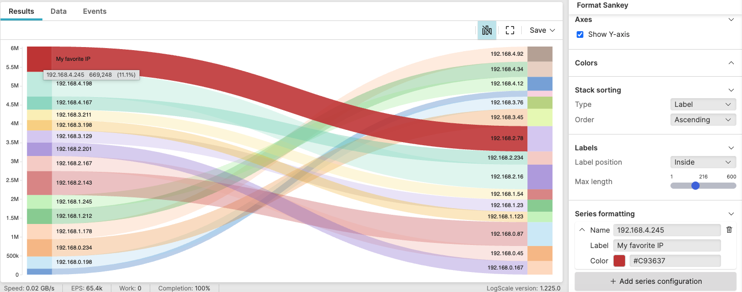 |
Figure 241. Network Traffic
Sample input data:
| dst_ip | pkt_size | protocol | src_ip | timestamp |
|---|---|---|---|---|
| 10.0.0.50 | 1500 | TCP | 192.168.1.100 | 2025-08-11T00:01:23Z |
| 10.0.0.51 | 2000 | UDP | 192.168.1.100 | 2025-08-11T00:01:24Z |
| 10.0.0.50 | 1000 | TCP | 192.168.1.101 | 2025-08-11T00:01:25Z |
| 10.0.0.52 | 3000 | TCP | 192.168.1.102 | 2025-08-11T00:01:26Z |
| 10.0.0.50 | 1800 | UDP | 192.168.1.100 | 2025-08-11T00:01:27Z |
Query:
sankey(source=src_ip, target=dst_ip, weight=sum(pkt_size))Query breakdown:
The
sankey()function takes source IP addresses as the starting nodes and destination IP addresses as the ending (target) nodes.Aggregates the total packet size for each source-destination pair. The sum of packet sizes determines the edge thickness (thicker lines = more data transferred).
Configuration:
From the
Searchpage, type your query in the Query Editor → clickChoose in the Widget selector
Click the style icon : this opens the Format panel on the side where some properties are already configured by default based on the query result.
Modify the properties to obtain the look and feel in this example, such as:
Set Stack sorting as
labelto show the series sorted by label name. Sorting them bysizeinstead will create a diagram that looks like this: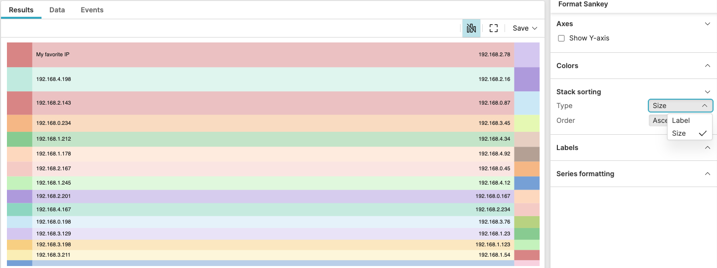
Figure 242. Network Traffic Visualization per Size
Keep the labels inside the diagram by setting Label position as
inside.In Series formatting, choose red as the color for series you particularly want to highlight.
You can further customize this widget by setting more properties, see Sankey Property Reference.