
Used with timeChart() or
bucket(), computes the aggregate for one or
more fields over a sliding window of preceding buckets. The
window looks backward from each bucket, excluding the current
bucket where the result is written. This function can only be
used as the function argument with
timeChart() or
bucket(). If used elsewhere, an error is
reported to the user.
| Parameter | Type | Required | Default Value | Description |
|---|---|---|---|---|
buckets | integer | optional[a] | Defines the number of buckets in the sliding time window, for example, the number of buckets in the surrounding timeChart() or bucket() to use for the running window aggregate. Exactly one of span and buckets should be defined. | |
function[b] | array of aggregate functions | optional[a] | count(as=_count) | Specifies which aggregate functions to perform on each window. If several aggregators are listed for the function parameter, then their outputs are combined using the rules described for stats(). |
span | long | optional[a] | Defines the width of the sliding time window. This value is rounded to the nearest multiple of time buckets of the surrounding timeChart() or bucket(). The time span is defined as a Relative Time Syntax like 1 hour or 3 weeks. If the query's time interval is less than the span of the window, no window result is computed. Exactly one of span and buckets should be defined. | |
[a] Optional parameters use their default value unless explicitly set. | ||||
Hide omitted argument names for this function
Omitted Argument NamesThe argument name for
functioncan be omitted; the following forms of this function are equivalent:logscale Syntaxwindow("value")and:
logscale Syntaxwindow(function="value")These examples show basic structure only.
window() Function Operation
The window() computes the running
aggregate (for example, avg() or
sum()) for the given incoming events. For
each window, the window() takes the
buckets parameter
and uses this to calculate the rolling aggregate across that
number of buckets in the input.
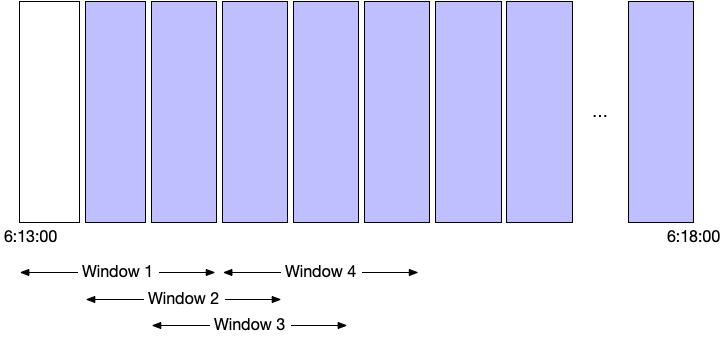
For example, this query calculates the rolling average over the preceding three buckets in the humio for allocBytes:
timeChart(span=15s,function=window(function=avg(allocBytes), buckets=3))
| formatTime(field=_bucket,format="%T",as=fmttime)
Tip
Use the Data tab in
Time Chart to view the raw
data being used for the chart.
| _bucket | _avg | fmttime |
|---|---|---|
| 1711520025000 | 18410.014084507042 | 06:13:45 |
| 1711520040000 | 23895.214188267393 | 06:14:00 |
| 1711520055000 | 24428.83897158322 | 06:14:15 |
| 1711520070000 | 24178.220994475138 | 06:14:30 |
| 1711520085000 | 24718.239339752407 | 06:14:45 |
| 1711520100000 | 18554.22950819672 | 06:15:00 |
| 1711520115000 | 25638.98775510204 | 06:15:15 |
| 1711520130000 | 18482.970792767734 | 06:15:30 |
| 1711520145000 | 25925.13892709766 | 06:15:45 |
| 1711520160000 | 19303.472527472528 | 06:16:00 |
| 1711520175000 | 25806.04081632653 | 06:16:15 |
| 1711520190000 | 17668.755244755244 | 06:16:30 |
| 1711520205000 | 24431.551299589602 | 06:16:45 |
| 1711520220000 | 17237.956043956045 | 06:17:00 |
| 1711520235000 | 23476.795669824085 | 06:17:15 |
| 1711520250000 | 15585.57082748948 | 06:17:30 |
| 1711520265000 | 22664.589358799454 | 06:17:45 |
| 1711520280000 | 16099.04132231405 | 06:18:00 |
A graphical representation, showing the span of each computed window is shown below.
 |
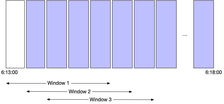
By comparison this query computes the value over the preceding 5 buckets:
timeChart(span=15s,function=window(function=avg(allocBytes), buckets=3))
| formatTime(field=_bucket,format="%T",as=fmttime)
The computed average is different because a different series of values in different buckets is being used to compute the value:
| _bucket | _avg | fmttime |
|---|---|---|
| 1711520025000 | 17772.622950819674 | 06:13:45 |
| 1711520040000 | 21970.357963875205 | 06:14:00 |
| 1711520055000 | 22170.04451772465 | 06:14:15 |
| 1711520070000 | 22505.86600496278 | 06:14:30 |
| 1711520085000 | 23378.47308319739 | 06:14:45 |
| 1711520100000 | 23568.354098360654 | 06:15:00 |
| 1711520115000 | 23566.52023121387 | 06:15:15 |
| 1711520130000 | 19816.212271973465 | 06:15:30 |
| 1711520145000 | 24608.287816843826 | 06:15:45 |
| 1711520160000 | 20315.036303630364 | 06:16:00 |
| 1711520175000 | 24221.750206782464 | 06:16:15 |
| 1711520190000 | 19854.064837905236 | 06:16:30 |
| 1711520205000 | 23849.69934640523 | 06:16:45 |
| 1711520220000 | 18996.489256198347 | 06:17:00 |
| 1711520235000 | 22389.50906095552 | 06:17:15 |
| 1711520250000 | 17751.334442595675 | 06:17:30 |
| 1711520265000 | 21959.068403908794 | 06:17:45 |
| 1711520280000 | 17377.422663358146 | 06:18:00 |
This can be represented graphically like this:
 |
If the number of buckets required by the sliding window to
compute its aggregate result is higher than the number of
buckets provided by the surrounding
timeChart() or
bucket() function, then the
window() function will yield an empty
result.
Any aggregate function can be used to compute sliding window data.
An example use case would be to find outliers, comparing a running average +/- running standard deviations to the concrete min/max values. This can be obtained by computing like this, which graphs the max value vs the limit value computed as average plus two standard deviations over the previous 15 minutes.
| timeChart(function=[max(m1),window([stdDev(m1),avg(m1)], span=15min)])
| groupBy(_bucket, function={ limit := _avg+2*_stddev
| table([_max, limit]) })
window() Examples
Click next to an example below to get the full details.
Make Data Compatible With Time Chart Widget - Example 1
Make data compatible with
Time Chart Widget using the
timeChart() function with
window() and
span parameter
Query
timeChart(host, function=window( function=avg(cpu_load), span=15min))Introduction
In this example, the timeChart() function is used
to create the required input format for the
Time Chart Widget and the
window() function is used to compute the running
aggregate (avg()) for the
cpu_load field over a sliding
window of data in the time chart. The span width, for example 15
minutes, is defined by the
span parameter. This defines
the duration of the average calculation of the input data, the average
value over 15 minutes. The number of buckets created will depend on the
time interval of the query. A 2 hour time interval would create 8
buckets.
Step-by-Step
Starting with the source repository events.
- logscale
timeChart(host, function=window( function=avg(cpu_load), span=15min))Groups by host, and calculates the average CPU load time per each 15 minutes over the last 24 hours for each host, displaying the results in a Time Chart Widget.
The running average time of CPU load is grouped into spans of 30 minutes. Note that the time interval of the query must be larger than the window span to produce any result.
Event Result set.
Summary and Results
Selecting the number of buckets or the timespan of each bucket enables you to show a consistent view either by time or by number of buckets independent of the time interval of the query. For example, the widget could show 10 buckets whether displaying 15 minutes or 15 days of data; alternatively the display could always show the data for each 15 minutes.
The query is used to make CPU load data compatible with the Time Chart Widget. This query is, for example, useful for CPU load monitoring to identify sustained high CPU usage over specific time periods.
For an example of dividing the input data by the number of buckets, see Make Data Compatible With Time Chart Widget - Example 2.
Make Data Compatible With Time Chart Widget - Example 2
Make data compatible with
Time Chart Widget using the
timeChart() function with
window() and
buckets parameter
Query
timeChart(host, function=window( function=[avg(cpu_load), max(cpu_load)], buckets=3))Introduction
In this example, the window() function uses the
number of buckets to calculate average and maximum CPU load. The
timespan for each bucket will depend on the time interval of the query.
The number of buckets are defined by the
buckets parameter. The
timeChart() function is used to create the required
input format for the Time Chart Widget.
The query calculates both average AND maximum values across the requested timespan. In this example, the number of buckets is specified, so the events will be distributed across the specified number of buckets using a time span calculated from the time interval of the query. For example, a 15 minute time interval with 3 buckets would use a timespan of 5 minutes per bucket.
Step-by-Step
Starting with the source repository events.
- logscale
timeChart(host, function=window( function=[avg(cpu_load), max(cpu_load)], buckets=3))Groups by host, and calculates both the average of CPU load time and the maximum CPU load time (using aggregates (
avg()andmax()) for the cpu_load field), displaying the results in 5 buckets showing a stacked graph for each host using a Time Chart Widget. Event Result set.
Summary and Results
Selecting the number of buckets or the timespan of each bucket enables you to show a consistent view either by time or by number of buckets independent of the time interval of the query. For example, the widget could show 10 buckets whether displaying 15 minutes or 15 days of data; alternatively the display could always show the data for each 15 minutes.
The query is used to make CPU load data compatible with the Time Chart Widget. This query is, for example, useful for CPU load monitoring to compare intervals, compare hourly performance etc.
For an example of dividing the input data by the timespan of each bucket, see Make Data Compatible With Time Chart Widget - Example 1.