The Scatter Chart is meant to be used in conjunction with functions such as table() select(), groupBy(), timeChart(), bucket(), and top().

For example, with a service producing logs like this:

2022-03-14T10:59:02.387+0000 INFO c.h.u.TimerExecutor$ 3 cputime=266935 wallclock=269564 alloc=4712
2022-03-14T10:59:02.389+0000 INFO c.h.u.TimerExecutor$ 1 cputime=17521 wallclock=19430 alloc=40
2022-03-14T10:59:02.419+0000 INFO c.h.u.TimerExecutor$ 3 cputime=95658 wallclock=98754 alloc=64

A chart can show the correlation between cputime, wallclock and memory allocation alloc using the table() function:

table([cputime, wallclock, alloc])

This query will produce a Scatter Chart with cputime as the X-axis and wallclock and alloc as two series of plotted numerical values (similar to Figure 213, “Scatter Chart”). Any additional inputs to the table() function field list would add more series to the chart.

Wide or long input format

The Input Data Format property is available in the Scatter Chart widget: when set to Auto mode, the chart looks at the query result and automatically chooses the best interpretation of the data between long or wide data format.

• Long format data must have one group field for the series names and two additional fields for x and y values respectively.

• Wide format must have at least two fields (neither needs to be a group field), the first one is used for x values and any subsequent fields contain y values. There is a limit of 49 series when the wide format is chosen (50 in total, but the x axis takes the first slot).

Notice that a group field is the field used as the first argument to either groupBy(), bucket() or timeChart() functions.

See an example of Auto mode that automatically selects the long data format, using a nested groupBy() function:

logscale

groupBy(#vhost, function=[groupBy(alloc)])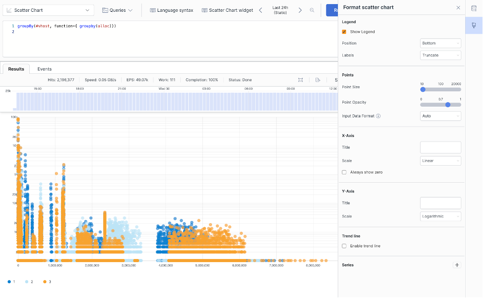

Figure 214. Scatter Chart Selecting Long Format