
The accumulate() function applies an
aggregation function cumulatively to a sequence of events. It is
useful for calculating running totals, running averages, or
other cumulative metrics over time or across a series of events.
For more information about sequence functions and combined usage, see Sequence Query Functions.
| Parameter | Type | Required | Default Value | Description |
|---|---|---|---|---|
current | enum | optional[a] | include | Controls whether to include the current event in the accumulation. |
| Values | ||||
exclude | Exclude current event in the accumulation | |||
include | Include current event in the accumulation | |||
function[b] | array of aggregate functions | required | The aggregator function to accumulate (for example, sum(), avg(), count()). It only accepts functions that output at most a single event. | |
[a] Optional parameters use their default value unless explicitly set. | ||||
Hide omitted argument names for this function
Omitted Argument NamesThe argument name for
functioncan be omitted; the following forms of this function are equivalent:logscale Syntaxaccumulate("value")and:
logscale Syntaxaccumulate(function="value")These examples show basic structure only.
accumulate() Function Operation
accumulate() has the following
operational behaviours:
The
accumulate()function must be used after an aggregator function (for example,head(),sort(),bucket(),groupBy()timeChart()) to ensure event ordering, as theaccumulate()function requires a specific order to calculate cumulative values correctly.Only functions (for example,
sum(),avg(),count()) that output a single event can be used in the sub-aggregation because theaccumulate()function needs a single value to add to its running total for each event.
accumulate() Examples
Click next to an example below to get the full details.
Calculate Running Average of Field Values
Calculate a running average of values in a dataset using the
accumulate() function
Query
head()
| accumulate(avg(value))
Introduction
In this example, the accumulate() function is used
with the avg() function to calculate a running
average of the field value.
Note that the accumulate() function must be used
after an aggregator function, in this example the
head() function, to ensure event ordering.
Example incoming data might look like this:
| key | value |
|---|---|
| a | 5 |
| b | 6 |
| c | 1 |
| d | 2 |
Step-by-Step
Starting with the source repository events.
- logscale
head()Ensures that the events are ordered by time, selecting the oldest events.
- logscale
| accumulate(avg(value))Computes the running average of all values, including the current one, using the
accumulate()function with theavg()aggregator. Event Result set.
Summary and Results
The query is used to calculate the running average of fields. The query calculates moving averages that change as new values arrive.
Sample output from the incoming example data:
| _avg | key | value |
|---|---|---|
| 5 | a | 5 |
| 5.5 | b | 6 |
| 4 | c | 1 |
| 3.5 | d | 2 |
Compute Cumulative Aggregation Across Buckets
Compute a cumulative aggregation across buckets using the
accumulate() function with
timeChart()
Query
timeChart(span=1000ms, function=sum(value))
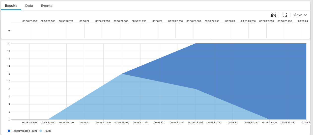
| accumulate(sum(_sum, as=_accumulated_sum))Introduction
In this example, the accumulate() function is used
with timeChart() to accumulate values across time
intervals.
Note that the accumulate() function must be used
after an aggregator function to ensure event ordering.
Example incoming data might look like this:
| @timestamp | key | value |
|---|---|---|
| 1451606301001 | a | 5 |
| 1451606301500 | b | 6 |
| 1451606301701 | a | 1 |
| 1451606302001 | c | 2 |
| 1451606302201 | b | 6 |
Step-by-Step
Starting with the source repository events.
- logscale
timeChart(span=1000ms, function=sum(value))Groups data into 1-second buckets over a 4-second period, sums the field value for each bucket and returns the results in a field named _sum. The result is displayed in a timechart.
- logscale
| accumulate(sum(_sum, as=_accumulated_sum))Calculates a running total of the sums in the _sum field, and returns the results in a field named _accumulated_sum.
Event Result set.
Summary and Results
The query is used to accumulate values across time intervals/buckets. The query is useful for tracking cumulative metrics or identifying trends in the data.
Sample output from the incoming example data:
| _bucket | _sum | _accumulated_sum |
|---|---|---|
| 1451606300000 | 0 | 0 |
| 1451606301000 | 12 | 12 |
| 1451606302000 | 8 | 20 |
| 1451606303000 | 0 | 20 |
The timechart looks like this:
 |
Compute Cumulative Aggregation For Specific Group
Compute a cumulative aggregation for a specific group using the
accumulate() function with
groupBy()
Query
head()
| groupBy(key, function = accumulate(sum(value)))
Introduction
In this example, to compute a cumulative aggregation for a specific
group (for example, by user), the accumulate()
function is used inside the groupBy() function.
Note that the accumulate() function must be used
after an aggregator function to ensure event ordering.
Example incoming data might look like this:
| key | value |
|---|---|
| a | 5 |
| b | 6 |
| a | 1 |
| c | 2 |
| b | 6 |
Step-by-Step
Starting with the source repository events.
- logscale
head()Selects the oldest events ordered by time.
- logscale
| groupBy(key, function = accumulate(sum(value)))Accumulates the sum of a field named value, groups the data by a specified key and returns the results in a field named _sum.
Event Result set.
Summary and Results
The query is used to compute a cumulative aggregation for a specific group, in this example using the value field.
Sample output from the incoming example data:
| key | _sum | value |
|---|---|---|
| a | 5 | 5 |
| a | 6 | 1 |
| b | 6 | 6 |
| b | 12 | 6 |
| c | 2 | 2 |
Count Events Within Partitions Based on Condition
Count events within partitions based on a specific condition using
the partition() function combined with
neighbor() and
accumulate()
Query
head()
| neighbor(key, prefix=prev)
| partition(accumulate(count()), condition=test(key != prev.key))
Introduction
Accumulations can be partitioned based on a condition, such as a change
in value. This is achieved by combining the three functions
partition(), neighbor() and
accumulate(). In this example, the combination of
the 3 sequence functions is used to count events within partitions
defined by changes in a key
field.
Note that sequence functions must be used after an aggregator function to ensure event ordering.
Example incoming data might look like this:
| key |
|---|
| a |
| a |
| a |
| b |
| a |
| b |
| b |
Step-by-Step
Starting with the source repository events.
- logscale
head()Selects the oldest events ordered by time.
- logscale
| neighbor(key, prefix=prev)Accesses the value in the field key from the previous event.
- logscale
| partition(accumulate(count()), condition=test(key != prev.key))The
partition()function splits the sequence of events based on the specified condition. A new partition starts when the current key value is different from the previous key value. Within each partition, it counts the number of events, and returns the results in a field named _count. Event Result set.
Summary and Results
The query is used to compute an accumulated count of events within partitions based on a specific condition, in this example change in value for the field key.
Sample output from the incoming example data:
| key | _count | prev.key |
|---|---|---|
| a | 1 | <no value> |
| a | 2 | a |
| a | 3 | a |
| b | 1 | a |
| a | 1 | b |
| b | 1 | a |
| b | 2 | b |
The query is useful for analyzing sequences of events, especially when you want to identify and count consecutive occurrences of a particular attribute in order to identify and analyze patterns or sequences within your data.
Detect Changes And Compute Differences Between Events - Example 2
Detect changes and compute differences between events using the
neighbor() function combined with
accumulate()
Query
head()
| neighbor(start, prefix=prev)
| duration := start - prev.start
| accumulate(sum(duration, as=accumulated_duration))
Introduction
In this example, the neighbor() function is used
with accumulate() to calculate a running total of
durations.
Note that the neighbor() function must be used
after an aggregator function to ensure event ordering.
Example incoming data might look like this:
| start |
|---|
| 1100 |
| 1233 |
| 3002 |
| 4324 |
Step-by-Step
Starting with the source repository events.
- logscale
head()Selects the oldest events ordered by time.
- logscale
| neighbor(start, prefix=prev)Retrieves the value in the start field from preceeding event, and assigns this value to the current event's data in a new field named prev.start.
- logscale
| duration := start - prev.startCalculates the time difference between current and previous start values, and returns the results - the calculated difference - in a field named duration.
- logscale
| accumulate(sum(duration, as=accumulated_duration))Calculates a running total sum of the values in the field duration and returns the results in a field named accumulated_duration. Each event will show its individual duration and the total accumulated duration up to that point.
Event Result set.
Summary and Results
The query is used to calculate the time difference between consecutive events. The format of this query is a useful pattern when analyzing temporal data, to provide insights into process efficiency, system performance over time etc. In this example, the acculated_duration provides a value that can be used to compare against the duration field within each event.
Sample output from the incoming example data:
| start | accumulated_duration | duration | prev.start |
|---|---|---|---|
| 1100 | 0 | <no value> | <no value> |
| 1233 | 133 | 133 | 1100 |
| 3002 | 1902 | 1769 | 1233 |
| 4324 | 3224 | 1322 | 3002 |
For example, in the results, the third event shows a large increase in duration against the accumulated_duration and the start time of the previous event (in prev.start). If analyzing execution times of a process, this could indicate a fault or delay compared to previous executions.