
Draw a Time Chart where the
x-axis is time. Time is grouped into buckets.
| Parameter | Type | Required | Default Value | Description |
|---|---|---|---|---|
buckets | number | optional[a] | Defines the number of buckets. The time span is defined by splitting the query time interval into this many buckets. | |
| Minimum | 1 | |||
| Maximum | 1500 | |||
function | array of aggregate functions | optional[a] | count() | Specifies which aggregate functions to perform on each group. If several aggregators are listed for the function parameter, then their outputs are combined using the rules described for stats(). |
limit | number | optional[a] | 10 | Defines the maximum number of series to produce. A warning is produced if this limit is exceeded, unless the parameter is specified explicitly. It prioritizes the top-N series. The top N value being the series with the highest numerical value attributed to it by the subquery across all fields. |
| Maximum | 500 | |||
minSpan | string | optional[a] | Determines the minimum span or size of the buckets that can be produced by timeChart(): for example, if set to 5h, a query duration of 1 day (24 hours), can only be split into 5 buckets, with the last bucket covering an additional hour into the future. Relative Time Syntax values are valid values for this parameter. | |
series[b] | string | optional[a] | Each value in the field specified by this parameter becomes a series on the graph. | |
span | string | optional[a] | auto | Defines the time span for each bucket. The time span is defined as a Relative Time Syntax like 1hour or 3 weeks— however, Anchoring to Specific Time Units is not supported when defining the time span. If not provided or set to auto, the search time interval, and thus the number of buckets, is determined dynamically. |
timezone | string | optional[a] | Defines the time zone for bucketing. This value overrides timeZoneOffsetMinutes which may be passed in the HTTP/JSON query API. For example: timezone=UTC or timezone='+02:00'. | |
unit | string | optional[a] | No conversion | Each value is a unit conversion for the given column. For instance: bytes/span to Kbytes/day converts a sum of bytes into Kb/day automatically taking the time span into account. If present, this array must be either length 1 (apply to all series) or have the same length as the function parameter. See the reference at Relative Time Syntax. |
[a] Optional parameters use their default value unless explicitly set. | ||||
Hide omitted argument names for this function
Omitted Argument NamesThe argument name for
seriescan be omitted; the following forms of this function are equivalent:logscale SyntaxtimeChart("value")and:
logscale SyntaxtimeChart(series="value")These examples show basic structure only.
timeChart() Function Operation
The timeChart() function has specific
implementation and operational considerations, outlined below.
Important
Anchored time units not supported
You cannot use
Calendar-Based Units and
Anchoring to Specific Time Units to
define the span length in timeChart().
Series Selection in timeChart()
The selection is based on the aggregate numerical output across all specified functions and all time buckets, not the series identifiers themselves.
The limit
prioritizes the top-N series. The top N value being the
series with the highest numerical value attributed to it by
the subquery across all fields.
Series Selection Process:
The selection is based on the numerical values produced by the subquery/function.
It is not based on the series names.
When multiple functions are used, the function considers all values produced.
For different examples of top N series selection, see Find Top N Value of Series - Example 1 and Find Top N Value of Series - Example 2.
timeChart() Syntax Examples
Show the number of events per hour over the last 24 hours. We do this by selecting to search over the last 24 hours in the time selector in the UI, and then we tell the function to make each time bucket one hour long (with
span=1hour):logscaletimeChart(span=1h, function=count())The above creates 24 time buckets when we search over the last 24 hours, and all searched events get sorted into groups depending on the bucket they belong to (based on their @timestamp value). When all events have been divided up by time, the
count()function is run on each group, giving us the number of events per hour.Instead of counting all events together, you can also count different kinds of events. For example, you may want to count different kinds of HTTP methods used for requests in the logs. If those are stored in a field named method, you can use this field as a series:
logscaletimeChart(span=1h, function=count(), series=method)Instead of having one group of events per time bucket (as in the previous example), we will now get multiple groups: one group for every value of method that exists in the timespan we're searching in. So if we are still searching over a 24 hour period, and we have received only
GET,PUT, andPOSTrequests in that timespan, we will get three groups of events per bucket (because we have three different values for method).This means we end up with 72 groups of events. And every group contains only events which correspond to some time bucket and a specific value of method. Then
count()is run on each of these groups, to give us the number ofGETevents per hour,PUTevents per hour, andPOSTevents per hour.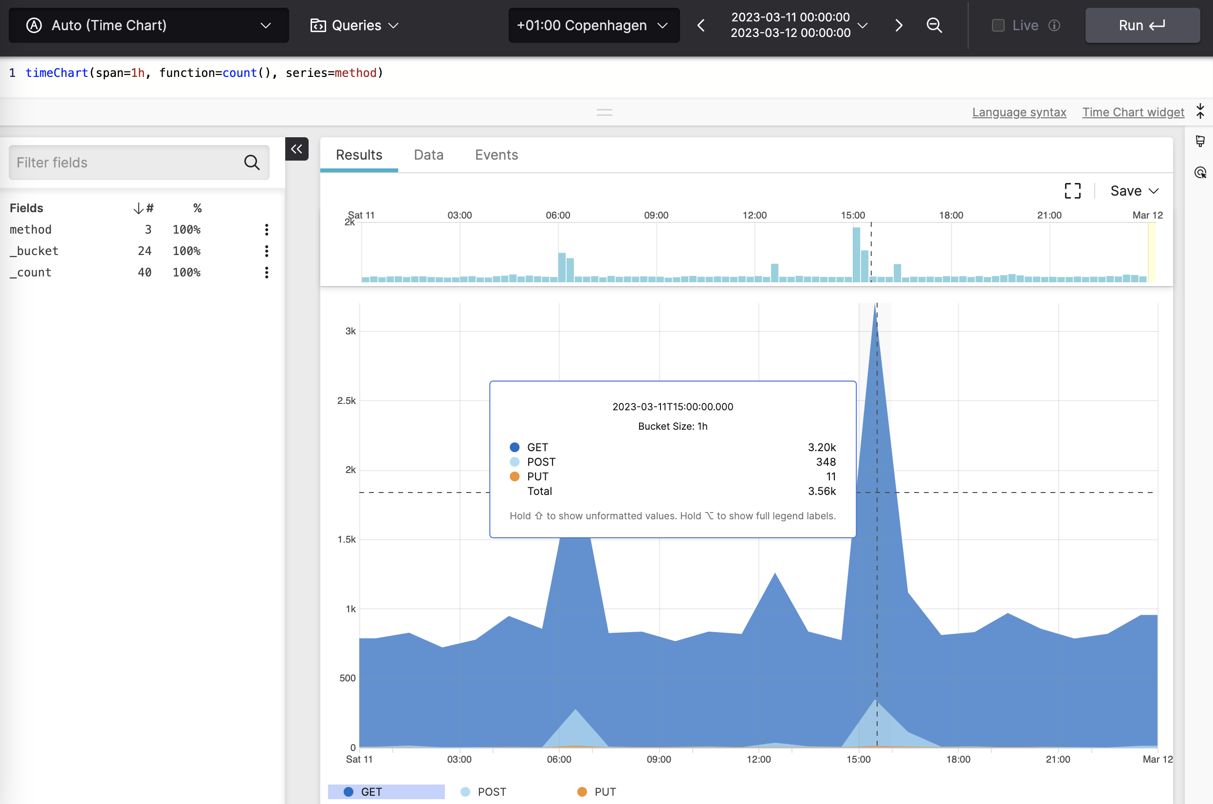
Figure 151. Counting Events Divided Into Buckets
Show the number of different HTTP methods by dividing events into time buckets of 1 minute and counting the HTTP methods (
GET,POST,PUTetc). As in the previous example, the timechart will have a line for each HTTP method.logscaletimeChart(span=1min, series=method, function=count())Use the number of buckets —instead of the time span — to show the number of different HTTP methods over time:
logscaletimeChart(buckets=1000, series=method, function=count())Get a graph with the response time percentiles:
logscaletimeChart(function=percentile(field=responsetime, percentiles=[50, 75, 90, 99, 99.9]))Use an array of functions in
functionto get a graph with the response time average as well as the percentiles:logscaletimeChart(function=[avg(responsetime), percentile(field=responsetime, percentiles=[50, 75, 90, 99, 99.9])])Use coda hale metrics to print rates of various events once per minute. Such lines include 1-minute average rates
m1=NwhereNis some number. This example displays all such meters (which are identified by the field name), converting the rates fromevents/sectoKi/day.logscaletype=METER rate_unit=events/second | timeChart(name, function=avg(m1), unit="events/sec to Ki/day", span=5m)Upon completion of every LogScale request, we issue a log entry which (among other things) prints the
size=Nof the result. When summing such size's you would need to be aware of the span, but using a unit conversion, we can display the number in Mbytes/hour, and the graph will be agnostic to the span.logscaletimeChart(function=sum(size), unit="bytes/bucket to Mbytes/hour", span=30m)
timeChart() Examples
Click next to an example below to get the full details.
Create Time Chart Widget for All Events
Query
timeChart(span=1h, function=count())Introduction
The Time Chart Widget is the most
commonly used widget in LogScale. It displays bucketed
time series data on a timeline. The
timeChart() function is used to create time
chart widgets, in this example a timechart that shows the number
of events per hour over the last 24 hours. We do this by selecting
to search over the last 24 hours in the time selector in the UI,
and then we tell the function to make each time bucket one hour
long (withspan=1hour).
Step-by-Step
Starting with the source repository events.
- logscale
timeChart(span=1h, function=count())Creates 24 time buckets when we search over the last 24 hours, and all searched events get sorted into groups depending on the bucket they belong to (based on their @timestamp value). When all events have been divided up by time, the
count()function is run on each group, giving us the number of events per hour. Event Result set.
Summary and Results
The query is used to create timechart widgets showing number of events per hour over the last 24 hours. The timechart shows one group of events per time bucket. When viewing and hovering over the buckets within the time chart, the display will show the precise value and time for the displayed bucket, with the time showing the point where the bucket starts.
Calculate a Percentage of Successful Status Codes Over Time
Convert status codes to success rate trends using the
if() function
Query
| success := if(status >= 500, then=0, else=1)
| timeChart(series=customer,function=
[
  {
    [sum(success,as=success),count(as=total)]
| pct_successful := (success/total)*100
| drop([success,total])}],span=15m,limit=100)
Introduction
Calculate a percentage of successful status codes inside the
timeChart() function field.
Step-by-Step
Starting with the source repository events.
- logscale
| success := if(status >= 500, then=0, else=1)Adds a success field at the following conditions:
If the value of field status is greater than or equal to
500, set the value of success to0, otherwise to1.
- logscale
| timeChart(series=customer,function=
[
  {
    [sum(success,as=success),count(as=total)]
Creates a new timechart, generating a new series, customer that uses a compound function. In this example, the embedded function is generating an array of values, but the array values are generated by an embedded aggregate. The embedded aggregate (defined using the
{}syntax), creates asum()andcount()value across the events grouped by the value of success field generated from the filter query. This is counting the11 or0generated by theif()function; counting all the values and adding up the ones for successful values. These values will be assigned to the success and total fields. Note that at this point we are still within the aggregate, so the two new fields are within the context of the aggregate, with each field being created for a corresponding success value. - logscale
| pct_successful := (success/total)*100Calculates the percentage that are successful. We are still within the aggregate, so the output of this process will be an embedded set of events with the total and success values grouped by each original HTTP response code.
- logscale
| drop([success,total])}],span=15m,limit=100)Still within the embedded aggregate, drop the total and success fields from the array generated by the aggregate. These fields were temporary to calculate the percentage of successful results, but are not needed in the array for generating the result set. Then, set a span for the buckets for the events of 15 minutes and limit to 100 results overall.
Event Result set.
Summary and Results
This query shows how an embedded aggregate can be used to generate a sequence of values that can be formatted (in this case to calculate percentages) and generate a new event series for the aggregate values.
Call Named Function on a Field - Example 2
Calls the named function (count()) on a field
over a set of events
Query
timeChart(function=[callFunction(?{function=count}, field=value)])Introduction
In this example, the callFunction() function is
used to call the named function (count()) on a
field over a set of events using the query parameter
?function.
Step-by-Step
Starting with the source repository events.
- logscale
timeChart(function=[callFunction(?{function=count}, field=value)])Counts the events in the value field, and displays the results in a timechart.
Notice how the query parameter
?functionis used to select the aggregation function for atimeChart(). Event Result set.
Summary and Results
The query is used to count events and chart them over time. Because we
are using callFunction(), it could be a different
function based on the dashboard parameter.
Using a query parameter (for example,
?function) to select the aggregation
function for a timeChart() is useful for dashboard
widgets.
Using callFunction() allow for using a function
based on the data or dashboard parameter instead of writing the query
directly.
Create Time Chart Widget for Different Events
Query
timeChart(span=1h, function=count(), series=method)Introduction
The Time Chart Widget is the most
commonly used widget in LogScale. It displays bucketed
time series data on a timeline. The
timeChart() function is used to create time
chart widgets, in this example a timechart that shows the number
of the different events per hour over the last 24 hours. For
example, you may want to count different kinds of HTTP methods
used for requests in the logs. If those are stored in a field
named method, you can use
this field as a series.
Furthermore, we select to search over the last 24 hours in the
time selector in the UI, and also add a function to make each time
bucket one hour long
(withspan=1hour).
Step-by-Step
Starting with the source repository events.
- logscale
timeChart(span=1h, function=count(), series=method)Creates 24 time buckets when we search over the last 24 hours, and all searched events get sorted into groups depending on the bucket they belong to (based on their @timestamp value). When all events have been divided up by time, the
count()function is run on the series field to return the number of each different kinds of events per hour. Event Result set.
Summary and Results
The query is used to create timechart widgets showing number of
different kinds of events per hour over the last 24 hours. In this
example we do not just have one group of events per time bucket, but
multiple groups: one group for every value of
method that exists in the
timespan we are searching in. So if we are still searching over a 24
hour period, and we have received only GET,
PUT, and POST requests
in that timespan, we will get three groups of events per bucket (because
we have three different values for
method) Therefore, we end up
with 72 groups of events. And every group contains only events which
correspond to some time bucket and a specific value of
method. Then
count() is run on each of these groups, to give us
the number of GET events per hour,
PUT events per hour, and
POST events per hour. When viewing and hovering
over the buckets within the time chart, the display will show the
precise value and time for the displayed bucket, with the time showing
the point where the bucket starts.
Create Time Chart With Default Percentiles For Multiple Fields
Visualize default percentiles (50th, 75th, 99th) of two metrics
over time using the percentile() function
with timeChart()
Query
timeChart(function=[percentile(field=r1,as=r1),percentile(field=r2,as=r2)], span=4m)Introduction
In this example, the timeChart() function combines
with two percentile() calculations to track the
distribution of two different metrics
(r1 and
r2) over time.
Note that when percentile() is used without
specifying percentiles, it automatically calculates three default
percentiles (50th, 75th, and 99th) for the given field.
Example incoming data might look like this:
| @timestamp | service | r1 | r2 | status |
|---|---|---|---|---|
| 2023-06-15T10:00:00Z | service_a | 120 | 150 | ok |
| 2023-06-15T10:01:00Z | service_a | 145 | 165 | ok |
| 2023-06-15T10:02:00Z | service_a | 98 | 110 | ok |
| 2023-06-15T10:03:00Z | service_a | 167 | 190 | error |
| 2023-06-15T10:04:00Z | service_a | 134 | 155 | ok |
| 2023-06-15T10:05:00Z | service_a | 178 | 195 | ok |
| 2023-06-15T10:06:00Z | service_a | 143 | 160 | ok |
| 2023-06-15T10:07:00Z | service_a | 156 | 175 | ok |
| 2023-06-15T10:08:00Z | service_a | 289 | 310 | error |
| 2023-06-15T10:09:00Z | service_a | 123 | 145 | ok |
Step-by-Step
Starting with the source repository events.
- logscale
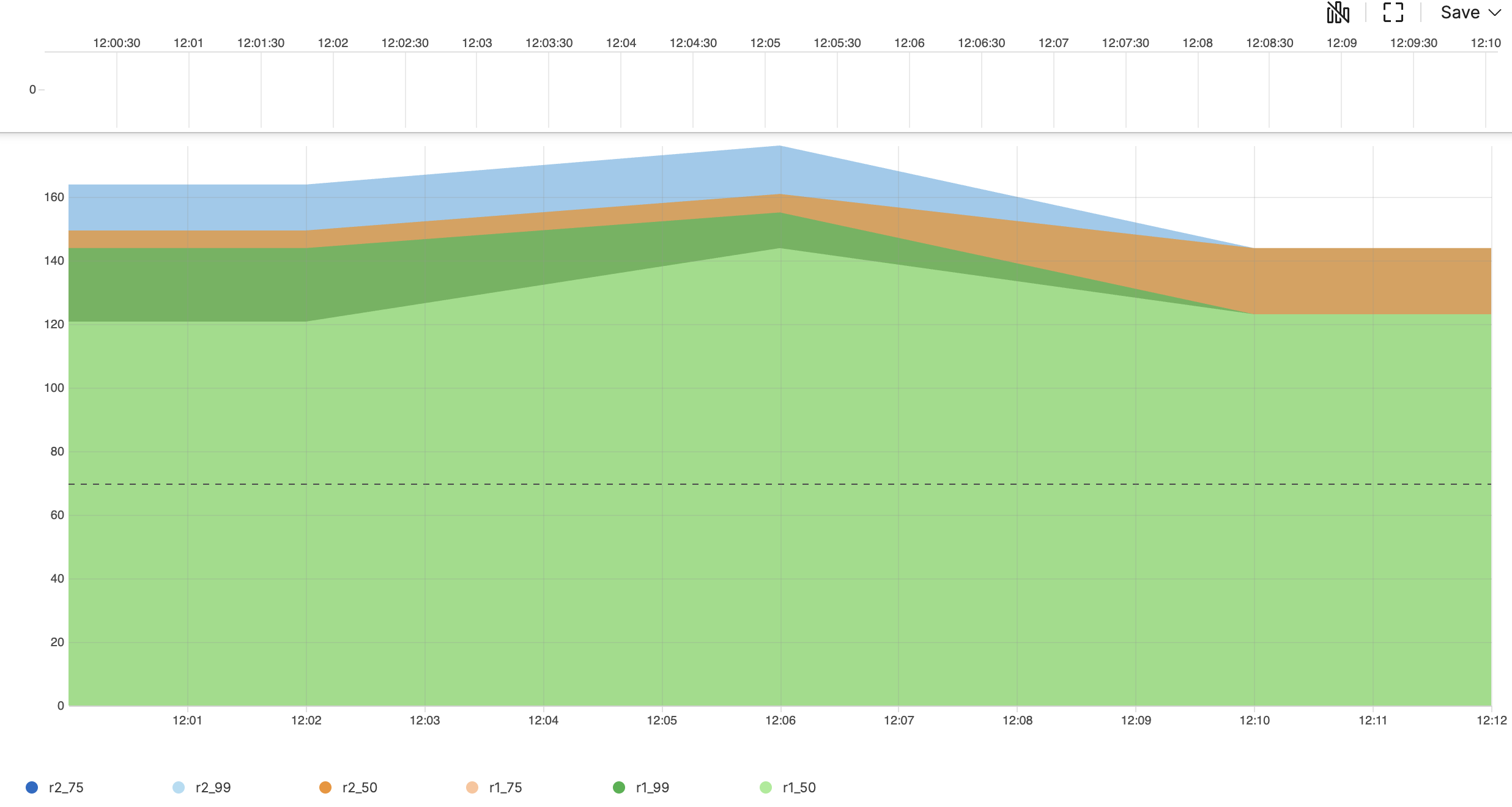
timeChart(function=[percentile(field=r1,as=r1),percentile(field=r2,as=r2)], span=4m)Creates a time chart with timespan of 4 minutes per bucket showing three percentile values for each field:
For field r1, creates:
r1_50 (median)
r1_75 (third quartile)
r1_99 (99th percentile)
For field r2, creates:
r2_50 (median)
r2_75 (third quartile)
r2_99 (99th percentile)
The
spanparameter is used to define the timespan of the bucket. Event Result set.
Summary and Results
The query produces a time series showing the distribution of both
metrics using three different percentile thresholds, allowing for
comprehensive performance analysis. When percentiles are not explicitly
specified, the percentile() function automatically
calculates three default percentiles (50th, 75th, and 95th).
This query is useful for comparing typical (median) performance between two metrics, identifying performance variations using the 75th percentile and monitoring extreme outliers with the 99th percentile
Sample output from the incoming example data:
| _bucket | r1_50 | r1_75 | r1_99 | r2_50 | r2_75 | r2_99 |
|---|---|---|---|---|---|---|
| 1.68682E+12 | 120.80792246242098 | 143.93947040702542 | 143.93947040702542 | 149.4847016559383 | 163.94784285493662 | 163.94784285493662 |
| 1.68682E+12 | 143.93947040702542 | 155.16205054702775 | 155.16205054702775 | 160.9814359681496 | 176.22889949490784 | 176.22889949490784 |
| 1.68682E+12 | 123.13088804780689 | 123.13088804780689 | 123.13088804780689 | 143.93947040702542 | 143.93947040702542 | 143.93947040702542 |
Note that the different buckets contain six different percentile values, three for each metric. The 99th percentile captures the extreme values in the data, making it useful for identifying outliers and performance anomalies.
 |
Create Time Chart With Fixed Bucket Count
Create a time chart with precise bucket control to visualize HTTP
Methods Distribution using timeChart()
function
Query
timeChart(buckets=10, series=method, function=count())Introduction
In this example, the timeChart() function is used
to create a time series visualization showing the distribution of HTTP
methods across exactly 10 time buckets.
Example incoming data might look like this:
| @timestamp | method | url | status_code | response_time |
|---|---|---|---|---|
| 2025-08-06T10:00:00Z | GET | /api/users | 200 | 45 |
| 2025-08-06T10:00:01Z | POST | /api/orders | 201 | 120 |
| 2025-08-06T10:00:02Z | GET | /api/products | 200 | 35 |
| 2025-08-06T10:00:03Z | PUT | /api/users/123 | 200 | 89 |
| 2025-08-06T10:00:04Z | DELETE | /api/orders/456 | 200 | 67 |
| 2025-08-06T10:00:05Z | GET | /api/inventory | 200 | 56 |
| 2025-08-06T10:00:06Z | POST | /api/users | 201 | 98 |
| 2025-08-06T10:00:07Z | GET | /api/orders | 200 | 43 |
| 2025-08-06T10:00:08Z | PATCH | /api/products/789 | 200 | 76 |
| 2025-08-06T10:00:09Z | GET | /api/status | 200 | 23 |
| 2025-08-06T10:00:10Z | HEAD | /api/health | 200 | 12 |
Step-by-Step
Starting with the source repository events.
- logscale
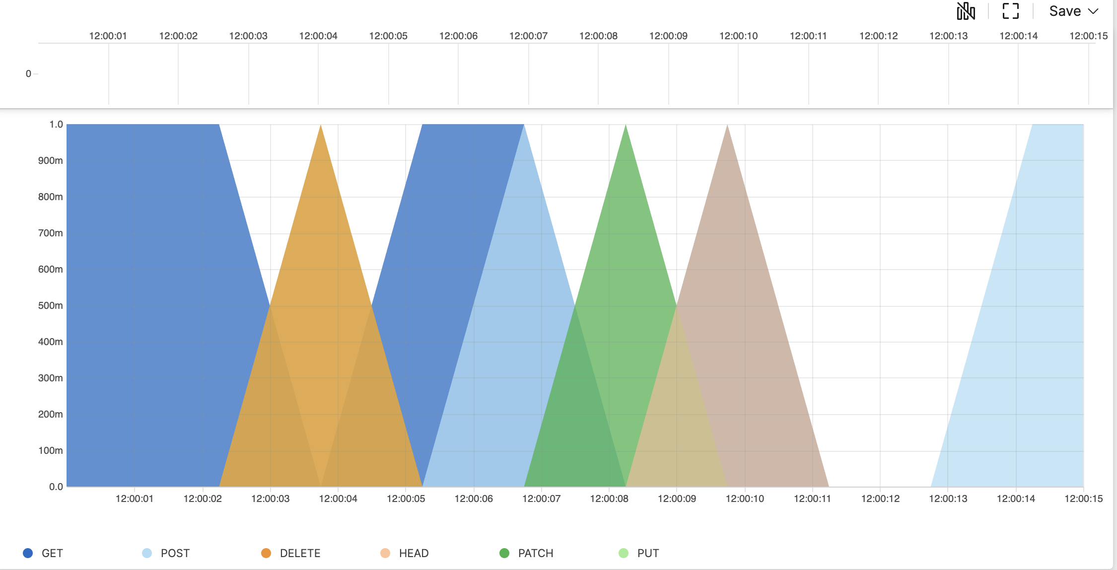
timeChart(buckets=10, series=method, function=count())Creates a time chart that divides the query time range into exactly 10 equal-width buckets.
The
seriesparameter groups the data by the method field, creating separate lines for each unique HTTP method.The
functionparameter usescount()to calculate the number of events in each bucket.Using
bucketsinstead of a time span ensures consistent granularity regardless of the total time range, making the visualization more predictable and easier to compare across different time ranges. For an example, see Create Time Chart With One-Minute Intervals. Event Result set.
Summary and Results
The query is used to create a detailed time series visualization showing how the usage of different HTTP methods varies over time, with precise control over the number of data points.
This query is useful, for example, to analyze API usage patterns, detect unusual spikes in specific HTTP methods, or monitor the distribution of request types with consistent granularity regardless of the time range.
If you want to create a time series visualization showing the
distribution of HTTP methods within the HUMIO repository,
you can use these queries: #kind=requests |
timeChart(buckets=10, series=method, function=count()) or just
#kind=requests | timeChart(series=method,
        function=count())
.
When the buckets
parameter is not specified, LogScale automatically determines an
appropriate number of buckets based on the query time range. This
ensures optimal visualization regardless of the time span being
analyzed.
Sample time chart from the incoming example data will look like this:
 |
Note that each HTTP method gets its own column, and the _bucket column represents the start of each time bucket. The values show the count of each method within that bucket.
Create Time Chart With One-Minute Intervals
Analyze request methods in fixed one-minute buckets using the
timeChart() function
Query
timeChart(span=1min, series=method, function=count())Introduction
In this example, the timeChart() function is used
with the span parameter
to create a time series visualization showing the count of HTTP request
methods aggregated into one-minute intervals.
Example incoming data might look like this:
| @timestamp | method | path | status_code | response_time |
|---|---|---|---|---|
| 2025-08-06T10:00:15Z | GET | /api/users | 200 | 45 |
| 2025-08-06T10:00:45Z | POST | /api/users | 201 | 78 |
| 2025-08-06T10:01:12Z | GET | /api/products | 200 | 32 |
| 2025-08-06T10:01:38Z | PUT | /api/users/1 | 200 | 65 |
| 2025-08-06T10:02:05Z | DELETE | /api/users/2 | 204 | 28 |
| 2025-08-06T10:02:30Z | GET | /api/orders | 200 | 52 |
| 2025-08-06T10:03:18Z | POST | /api/orders | 201 | 89 |
| 2025-08-06T10:03:42Z | GET | /api/products | 200 | 41 |
| 2025-08-06T10:04:15Z | PUT | /api/orders/1 | 200 | 67 |
| 2025-08-06T10:04:55Z | GET | /api/users | 200 | 38 |
Step-by-Step
Starting with the source repository events.
- logscale
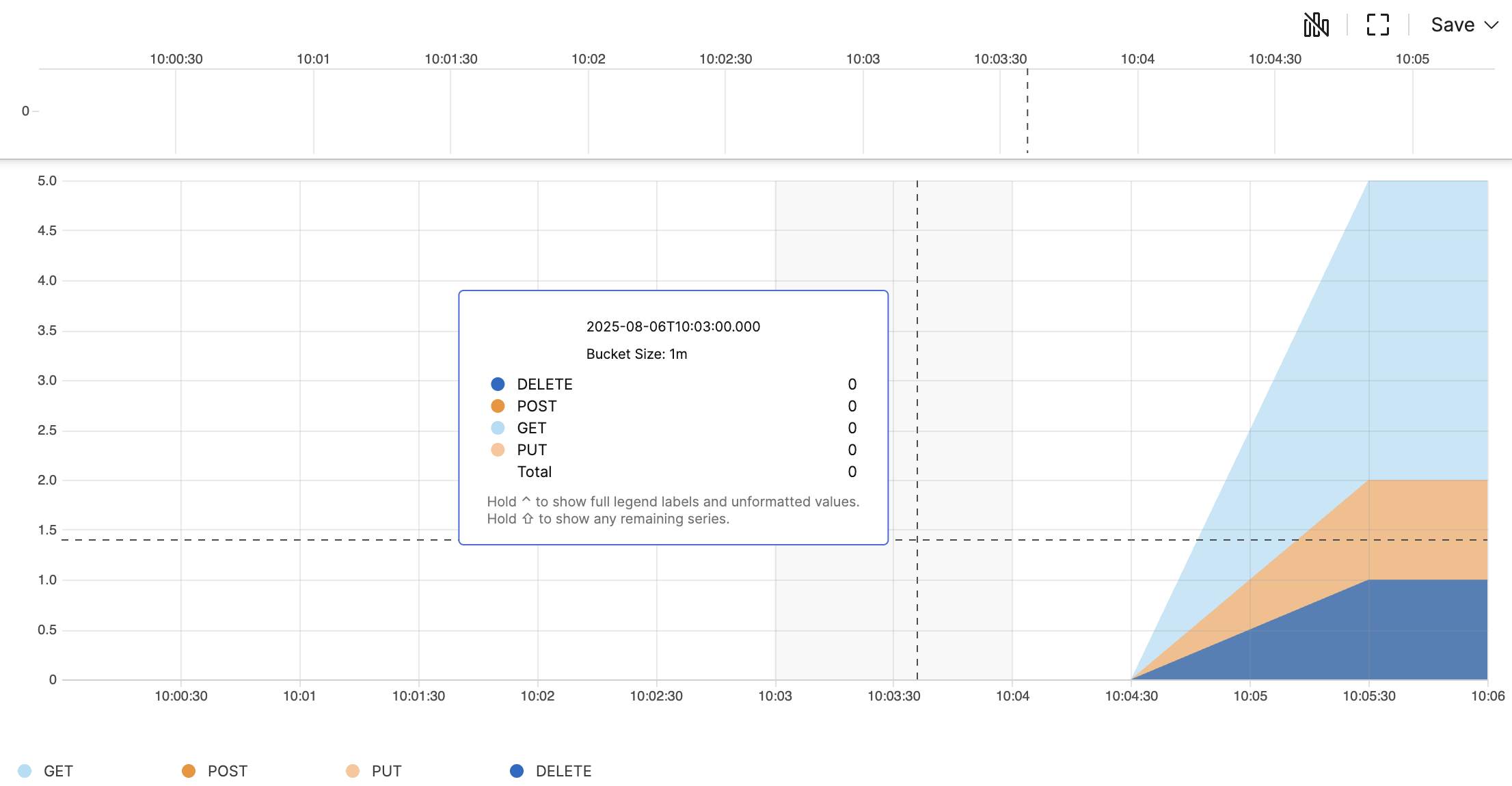
timeChart(span=1min, series=method, function=count())Creates a time series chart by grouping events into fixed one-minute intervals using
span=1minThe
seriesparameter groups the data by the method field, creating separate lines for each unique HTTP method.The
functionparameter usescount()to calculate the number of events in each minute interval for each method.The
spanparameter creates fixed-width time buckets, ensuring consistent interval sizes regardless of the query time range. This differs from usingbuckets, which divides the total time range into a specified number of intervals. For an example, see Create Time Chart With Fixed Bucket Count. Event Result set.
Summary and Results
The query is used to analyze the precise per-minute distribution of HTTP request methods, providing fixed time interval analysis.
This query is useful, for example, to monitor minute-by-minute API usage patterns, detect short-term spikes in specific request methods and analyze request patterns with consistent time granularity
If you want to create a time series visualization showing the
distribution of HTTP methods within the HUMIO repository,
you can use this query:#kind=requests |
timeChart(span=1min, series=method, function=count())
Sample time chart from the incoming example data will look like this:
 |
Note that events are grouped into the minute they occurred in, regardless of the specific seconds.
Find Top N Value of Series - Example 1
Find top N value of series using the
timeChart() function
Query
timeChart(series=key, function=max(value), limit=2)Introduction
In this example, the timeChart() function is used
to find the top 2 values of the
key series and display the
results in a Table Widget.
The limit parameter of
timeChart() prioritizes the top N series. The top N
value being the series with the highest numerical value attributed to it
by the subquery across all fields. The selection is based on the
numerical values produced by the subquery/function. When multiple
functions are used, it considers all values produced. The selection
process is not based on the series names (in this example
key).
Example incoming data might look like this:
| key | value |
|---|---|
| a | 42 |
| b | 41 |
| c | 40 |
Step-by-Step
Starting with the source repository events.
- logscale
timeChart(series=key, function=max(value), limit=2)Groups data by time using the key field as the series identifier (each unique key value becomes a separate series), then calculates the maximum value for each series.
Within each time bucket, it then takes highest calculated value for that key (series) and returns only the top 2 keys based on the calculated values in the new field named _max (generated by the
max()). Event Result set.
Summary and Results
The query is used to find the Top 2 value of series and display the
results in a Table Widget. In this
example, the top 2 series are a and
b, as they have the highest numerical value output by
the subquery (which is max() in this case).
This method can be used to provide a top N table or bar chart when looking for highest or lowest entries for a given query. The query can be used, for example, to track top 2 highest-performing metrics, to monitor highest resource consumers (CPU, memory), or to analyze top performers over time etc.
Sample output from the incoming example data:
| _bucket | key | _max |
|---|---|---|
| 1747109790000 | a | 42 |
| 1747109790000 | b | 41 |
The same input can output a different result if the
timeChart() function is used with multiple
functions. For more information, see
Find Top N Value of Series - Example 2.
Find Top N Value of Series - Example 2
Find top N value of series using the
timeChart() function with
max() and selectLast()
Query
timeChart(series=key, function=[max(value), {foo := value % 41 | selectLast(foo)}], limit=2)Introduction
In this example, the timeChart() function is used
with multiple functions and modulus operation to find the top 2 values
of the key series and display
the results in a Table Widget.
The limit parameter of
timeChart() prioritizes the top N series. The top N
value being the series with the highest numerical value attributed to it
by the subquery across all fields. The selection is based on the
numerical values produced by the subquery/function. When multiple
functions are used, it considers all values produced for the
corresponding key or keys selected by the
series parameter. In this
example values are calculated for the
foo value and
_max maximum value of the field.
The selection process is not based on the series values from the
key field.
Example incoming data might look like this:
| key | value |
|---|---|
| a | 42 |
| b | 41 |
| c | 40 |
Step-by-Step
Starting with the source repository events.
- logscale
timeChart(series=key, function=[max(value), {foo := value % 41 | selectLast(foo)}], limit=2)Groups data by time using the key field as the series identifier, then takes the maximum value and performs a modulus operation (represented by
% 41in the example) on the value, comparing that to the last value of foo using theselectLast()function. With a limit 2, only the top 2 results are displayed.The series selection is based on combined numerical output of both the
max()function and the calculation for foo.Note that each value is divided by
41and the modulus operator returns the remainder and stores it in the field foo. The modulus operation creates a new set of values that, combined withmax(value), determines which series have the highest total numerical values. The series selection is based on combined numerical output of both values.The modulus calculations in this example are as follows:
42 % 41 = 1 (42 divided by 41 = 1
              remainder 1, foo=1)
41 % 41 = 0 (41 divided by 41 = 1 remainder 0, foo=0)40 % 41 = 40 (40 divided by 41 = 0 remainder 40, foo=40)
Event Result set.
Summary and Results
The query is used to find top 2 value of series using multiple functions and display the results in a Table Widget. When multiple functions are used, it considers all values produced for each element in the series.
The top 2 series are (in this example with multiple functions used)
a and c, as the output of the
subquery is:
_max = 42, foo = 1  // for 'a', (total=43)
_max = 41, foo = 0  // for 'b', (total=41)
_max = 40, foo = 40 // for 'c', (total=80)
meaning a and c have the highest
combined numerical values and thus are the top series.
Note how c has higher total despite lower
max(). This is because all produced values are
considered and the result of the modulus calculation creates a higher
remainder and overall total.
The query can be used, for example, for advanced pattern detection to find series with interesting combinations of metrics, or for anomaly detection to identify unusual patterns using multiple calculations.
Sample output from the incoming example data:
| _bucket | key | _max | foo |
|---|---|---|---|
| 1747109790000 | a | 42 | 1 |
| 1747109790000 | c | 40 | 40 |
The same input can output a different result if the
timeChart() function is used with a single
aggregator function only. For more information, see
Find Top N Value of Series - Example 1.
Make Data Compatible With Time Chart Widget - Example 1
Make data compatible with
Time Chart Widget using the
timeChart() function with
window() and
span parameter
Query
timeChart(host, function=window( function=avg(cpu_load), span=15min))Introduction
In this example, the timeChart() function is used
to create the required input format for the
Time Chart Widget and the
window() function is used to compute the running
aggregate (avg()) for the
cpu_load field over a sliding
window of data in the time chart. The span width, for example 15
minutes, is defined by the
span parameter. This defines
the duration of the average calculation of the input data, the average
value over 15 minutes. The number of buckets created will depend on the
time interval of the query. A 2 hour time interval would create 8
buckets.
Step-by-Step
Starting with the source repository events.
- logscale
timeChart(host, function=window( function=avg(cpu_load), span=15min))Groups by host, and calculates the average CPU load time per each 15 minutes over the last 24 hours for each host, displaying the results in a Time Chart Widget.
The running average time of CPU load is grouped into spans of 30 minutes. Note that the time interval of the query must be larger than the window span to produce any result.
Event Result set.
Summary and Results
Selecting the number of buckets or the timespan of each bucket enables you to show a consistent view either by time or by number of buckets independent of the time interval of the query. For example, the widget could show 10 buckets whether displaying 15 minutes or 15 days of data; alternatively the display could always show the data for each 15 minutes.
The query is used to make CPU load data compatible with the Time Chart Widget. This query is, for example, useful for CPU load monitoring to identify sustained high CPU usage over specific time periods.
For an example of dividing the input data by the number of buckets, see Make Data Compatible With Time Chart Widget - Example 2.
Make Data Compatible With Time Chart Widget - Example 2
Make data compatible with
Time Chart Widget using the
timeChart() function with
window() and
buckets parameter
Query
timeChart(host, function=window( function=[avg(cpu_load), max(cpu_load)], buckets=3))Introduction
In this example, the window() function uses the
number of buckets to calculate average and maximum CPU load. The
timespan for each bucket will depend on the time interval of the query.
The number of buckets are defined by the
buckets parameter. The
timeChart() function is used to create the required
input format for the Time Chart Widget.
The query calculates both average AND maximum values across the requested timespan. In this example, the number of buckets is specified, so the events will be distributed across the specified number of buckets using a time span calculated from the time interval of the query. For example, a 15 minute time interval with 3 buckets would use a timespan of 5 minutes per bucket.
Step-by-Step
Starting with the source repository events.
- logscale
timeChart(host, function=window( function=[avg(cpu_load), max(cpu_load)], buckets=3))Groups by host, and calculates both the average of CPU load time and the maximum CPU load time (using aggregates (
avg()andmax()) for the cpu_load field), displaying the results in 5 buckets showing a stacked graph for each host using a Time Chart Widget. Event Result set.
Summary and Results
Selecting the number of buckets or the timespan of each bucket enables you to show a consistent view either by time or by number of buckets independent of the time interval of the query. For example, the widget could show 10 buckets whether displaying 15 minutes or 15 days of data; alternatively the display could always show the data for each 15 minutes.
The query is used to make CPU load data compatible with the Time Chart Widget. This query is, for example, useful for CPU load monitoring to compare intervals, compare hourly performance etc.
For an example of dividing the input data by the timespan of each bucket, see Make Data Compatible With Time Chart Widget - Example 1.
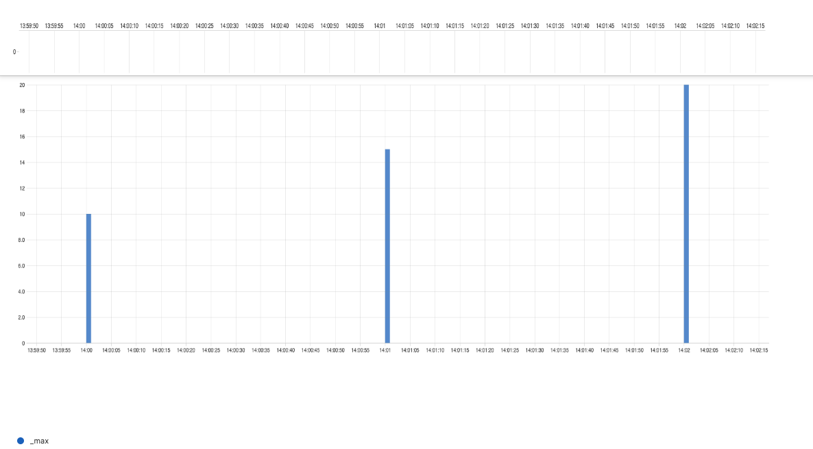
Rounding Within a Timechart
Round down a number in a field and display information in a
timechart using the round() and
timeChart() functions
Query
timeChart(function={max(value) | round(_max, how=floor)})timechart(function=max(value))Introduction
In this example, the round() function is used
with a floor parameter
to round down a field value to an integer (whole number) and
display information within a timechart.
Step-by-Step
Starting with the source repository events.
- logscale
timeChart(function={max(value) | round(_max, how=floor)})timechart(function=max(value))Creates a time chart using
max()as the aggregate function for a field named value to find the highest value in each time bucket, and returns the result in a field named _max.Rounds the implied field _max from the aggregate
max()using theflooroption to round down the value.Example of original _max values:
10.8,15.3,20.7.After floor:
10,15,20. Event Result set.
Summary and Results
The query is used to round down maximum values over time to nearest integer (whole value). This is useful when displaying information in a time chart. Rounding to nearest integer will make it easier to distinguish the differences between values when used on a graph for time-based visualization. The query simplifies the data presentation.
Note
To round to a specific decimal accuracy, the
format() function must be used.
 |