
Extends the groupBy() function for grouping by time,
diving the search time interval into buckets. Each event is put into a
bucket based on its timestamp.
When using the bucket() function, events are grouped
by a number of notional 'buckets', each defining a timespan, calculated by
dividing the time range by the number of required buckets. The function
creates a new field, _bucket, that
contains the corresponding bucket's start time in milliseconds (UTC time).
The bucket() function accepts the same parameters as
groupBy().
The output from the bucket() is a table and can be
used as the input for a variety of ???.
Alternatively, use the timeChart() function.
| Parameter | Type | Required | Default | Description |
|---|---|---|---|---|
buckets | number | optional[a] | Defines the number of buckets. The time span is defined by splitting the query time interval into this many buckets. 0..1500 | |
field | string | optional[a] | Specifies which fields to group by. Note it is possible to group by multiple fields. | |
function | Array of Aggregate Functions | optional[a] | count(as=_count) | Specifies which aggregate functions to perform on each group. Default is to count the elements in each group. |
limit | integer | optional[a] | 10 | Defines the maximum number of series to produce. A warning is produced if this limit is exceeded, unless the parameter is specified explicitly. |
| Maximum | 500 | |||
minSpan | long | optional[a] | It sets the minimum allowed span for each bucket, for cases where the buckets parameter has a high value and therefore the span of each bucket can be so small as to be of no use. It is defined as a Relative Time Syntax such as 1hour or 3 weeks. minSpan can be as long as the search interval at most — if set as longer instead, a warning notifies that the search interval is used as the minSpan. | |
span[b] | relative-time | optional[a] | auto | Defines the time span for each bucket. The time span is defined as a relative time modifier like 1hour or 3 weeks. If not provided or set to auto the search time interval, and thus the number of buckets, is determined dynamically. |
timezone | string | optional[a] | Defines the time zone for bucketing. This value overrides timeZoneOffsetMinutes which may be passed in the HTTP/JSON query API. For example, timezone=UTC or timezone='+02:00'. See the full list of timezones supported by LogScale at Supported Timezones. | |
unit | Array of strings | optional[a] | Each value is a unit conversion for the given column. For instance: bytes/span to Kbytes/day converts a sum of bytes into Kb/day automatically taking the time span into account. If present, this array must be either length 1 (apply to all series) or have the same length as function. | |
[a] Optional parameters use their default value unless explicitly set | ||||
Omitted Argument NamesThe argument name for
spancan be omitted; the following forms of this function are equivalent:logscalebucket("auto")and:
logscalebucket(span="auto")
When generating aggregated buckets against data, the exact number of buckets may not match the expected due to the combination of the query span, requested number of buckets, and available event data.
For example, given a query displaying buckets for every one minute, but with a query interval of 1 hour starting at 09:17:30, 61 buckets will be created, as represented by the shaded intervals shown in Figure 174, “Bucket Allocation using bucket()”:
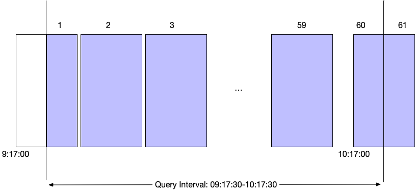 |
Figure 174. Bucket Allocation using bucket()
The buckets are generated, first based on the requested timespan interval or number of buckets, and then on the relevant timespan boundary. For example:
An interval per hour across a day will start at 00:00
An interval of a minute across an hour will start at 09:00:00
Buckets will contain the following event data:
The first bucket will contain the extracted event data for the relevant timespan (1 bucket per minute from 09:17), but only containing events after query interval. For example, the bucket will start 09:17, but contain only events with a timestamp after 09:17:30
The next 58 buckets will contain the event data for each minute.
Bucket 60 will contain the event data up until 10:17:30.
Bucket 61 will contain any remaining data from the last time interval bucket.
The result is that the number of buckets returned will be 61, even though
the interval is per minute across a one hour boundary. The trailing data
will always be included in the output. It may have an impact on the data
displayed when bucket() is used in combination with a
Time Chart.
bucket() Examples
Aggregating Status Codes by count() per minute
bucket(1min, field=status_code, function=count())Counts different HTTP status codes over time and buckets them into time intervals of 1 minute. Notice we group by two fields: status code and the implicit field _bucket.
Step-by-StepStarting with the source repository events
- flowchart LR; repo{{Events}} 0{{Aggregate}} result{{Result Set}} repo --> 0 0 --> result style 0 fill:#ff0000,stroke-width:4px,stroke:#000;
Set the bucket interval to 1 minute, aggregating the count of the field status_code.
logscalebucket(1min, field=status_code, function=count()) Event Result set
Bucketing allows for data to be collected according to a time
range. Using the right aggregation function to quantify the value
groups that information into the buckets suitable for graphing for
example with a Bar Chart, with the
size of the bar using the declared function result,
count() in this example.
Bucket Counts when using bucket()
Search Repository: humio-metrics
bucket(buckets=24, function=sum("count"))
| parseTimestamp(field=_bucket,format=millis)
When generating a list of buckets using the
bucket() function, the output will always
contain one more bucket than the number defined in
buckets. This is
to accommodate all the values that will fall outside the given
time frame across the requested number of buckets. This
calculation is due to the events being bound by the bucket in
which they have been stored, resulting in
bucket() selecting the buckets for the
given time range and any remainder. For example, when requesting
24 buckets over a period of one day in the
humio-metrics repository:
Starting with the source repository events
- flowchart LR; repo{{Events}} 0{{Aggregate}} 1>Augment Data] result{{Result Set}} repo --> 0 0 --> 1 1 --> result style 0 fill:#ff0000,stroke-width:4px,stroke:#000;
Bucket the events into 24 groups, using the
sum()function on the count field.logscalebucket(buckets=24, function=sum("count")) - flowchart LR; repo{{Events}} 0{{Aggregate}} 1>Augment Data] result{{Result Set}} repo --> 0 0 --> 1 1 --> result style 1 fill:#ff0000,stroke-width:4px,stroke:#000;
Extract the timestamp from the generated bucket and convert to a date time value; in this example the bucket outputs the timestamp as an epoch value in the _bucket field.
logscale| parseTimestamp(field=_bucket,format=millis) Event Result set
The resulting output shows 25 buckets, the original 24 requested one additional that contains all the data after the requested timespan for the requested number of buckets.
| _bucket | _sum | @timestamp |
|---|---|---|
| 1681290000000 | 1322658945428 | 1681290000000 |
| 1681293600000 | 1879891517753 | 1681293600000 |
| 1681297200000 | 1967566541025 | 1681297200000 |
| 1681300800000 | 2058848152111 | 1681300800000 |
| 1681304400000 | 2163576682259 | 1681304400000 |
| 1681308000000 | 2255771347658 | 1681308000000 |
| 1681311600000 | 2342791941872 | 1681311600000 |
| 1681315200000 | 2429639369980 | 1681315200000 |
| 1681318800000 | 2516589869179 | 1681318800000 |
| 1681322400000 | 2603409167993 | 1681322400000 |
| 1681326000000 | 2690189000694 | 1681326000000 |
| 1681329600000 | 2776920777654 | 1681329600000 |
| 1681333200000 | 2873523432202 | 1681333200000 |
| 1681336800000 | 2969865160869 | 1681336800000 |
| 1681340400000 | 3057623890645 | 1681340400000 |
| 1681344000000 | 3144632647026 | 1681344000000 |
| 1681347600000 | 3231759376472 | 1681347600000 |
| 1681351200000 | 3318929777092 | 1681351200000 |
| 1681354800000 | 3406027872076 | 1681354800000 |
| 1681358400000 | 3493085788508 | 1681358400000 |
| 1681362000000 | 3580128551694 | 1681362000000 |
| 1681365600000 | 3667150316470 | 1681365600000 |
| 1681369200000 | 3754207997997 | 1681369200000 |
| 1681372800000 | 3841234050532 | 1681372800000 |
| 1681376400000 | 1040019734927 | 1681376400000 |
Bucket Events summarized by count()
bucket(function=count())Divides the search time interval into buckets. As time span is not specified, the search interval is divided into 127 buckets. Events in each bucket are counted:
Step-by-StepStarting with the source repository events
- flowchart LR; repo{{Events}} 0{{Aggregate}} result{{Result Set}} repo --> 0 0 --> result style 0 fill:#ff0000,stroke-width:4px,stroke:#000;
Summarize events using the
count()into buckets across the selected timespan.logscalebucket(function=count()) Event Result set
This query organizes data into buckets according to the count of events.
Showing Percentiles across Multiple Buckets
bucket(span=60sec, function=percentile(field=responsetime, percentiles=[50, 75, 99, 99.9]))Show response time percentiles over time. Calculate percentiles per minute by bucketing into 1 minute intervals:
Step-by-StepStarting with the source repository events
- flowchart LR; repo{{Events}} 0{{Aggregate}} result{{Result Set}} repo --> 0 0 --> result style 0 fill:#ff0000,stroke-width:4px,stroke:#000;
Using a 60 second timespan for each bucket, display the
percentile()for the responsetime field.logscalebucket(span=60sec, function=percentile(field=responsetime, percentiles=[50, 75, 99, 99.9])) Event Result set
The percentile() quantifies values by
determining whether the value is larger than a percentage of the
overall values. The output provides a powerful view of the
relative significance of a value. Combined in this example with
bucket(), the query will generate buckets of
data showing the comparative response time for every 60 seconds.