
Search Architecture
LogScale search is designed around flexibility and being able to ask questions on data without necessarily knowing data structure, or the questions that might need to be asked when data is ingested. See Design Principles. LogScale tries to provide an efficient trade-off between ingesting the data efficiently and then providing the ability to search the data.
Temporal Data
LogScale is a temporal database. All data within LogScale is stored according to a timestamp (in the @timestamp field for every event). This temporal information determines how data is stored (in sequential segments) and where it is stored (most recent data on local disks, older data on object storage).
Whenever a search is performed, the search is always executed on the basis of a timespan, whether relative (last 5 minutes) or absolute (10:00am to 11:00am). All data is search and returned on this basis. The basic structure when searching for information is a sequence of events, ordered by the timestamp for each event.
Metadata
In Design Principles it was asserted that LogScale does not use indexes.
In fact, LogScale has some index like structures. LogScale treats this information as metadata and that data assists LogScale during search. LogScale uses the Global Database to share information about where data segments are stored. Segments define a series of data, organized by the datasource, which in turn is defined by one or more tags. The global database stores the segment data that correlates the tags and time spans to the segments. This metadata is the first element of metadata that allows LogScale to select a specific series of segment files to be used as the basis of the search.
In combination with the temporal nature of the data, LogScale is able to select a specific set of segments to read when searching for data.
For example, when executing the query:
#host=server3
| #source=loadbalance
With an interval of 11:01:30 to 11:00:00, LogScale uses the Global Database to identify two specific segments to search for events:
The segments in green are the segments that should be searched. If the segments are on the local disk, the search continues, but if the segments are on block storage, they are copied back from block storage to a storage node so that the stored events can be processed.
During this process, the Query Coordinator manages the processes, identifying where the segments are located, on which nodes the blocks exist (or have been copied to) and therefore which nodes will process the individual events.
Hash Filters
To avoid having to brute force scan all the relevant segments for a search, LogScale uses hash filters. Hashfilters are a form of filter built on top of Bloomfilters. For each segment file LogScale creates a hash file that is always placed alongside the segment, with segments and hashfilter filters being moved in tandem.
The hashfilter is used to limit the blocks within the segment file that needs to be read. This can create huge performance gains by limiting even further the blocks (and even entire segments) that need to be read and processed.
Hash filters work with both structured or unstructured data. Searching
for a freetext string will allow the hash filters to kick in and filter
which data that needs to be searched. Hash filters support finding
strings that exists everywhere in the event, even substrings in words.
When searching structure data, hashfilters can determine if the explicit
data exists in certain blocks. For example when searching for
statuscode=500 the hashfilter will
select only those matching blocks.
Hash filters have some anomalies, in that they can sometimes return false positives, but they are generally a reliable way of filtering out non-matching blocks.
To compare the effect of a hashfilter search to a non-hashfilter search:
Where hashfilters speed up the searching process
Some hashfilter scenarios:
Checking if an "evil" ip address has been seen anywhere on the network for the last month. A freetext search for the ip address over different datasources will be performed across multiple datasources. Without hashfilters LogScale would have to open every segments from every datasources over the last month. With a hashfilter, only the hashfilter files are opened and any blocks or segments that dont match the information will be filtered away.
Where hashfilters do not help is when the search ends up returning most
blocks, or when it creates a range search, for example
statuscode>=300.
Compression
As described in Ingestion: Digest Phase, LogScale compresses the segment files as they are stored on disk. Just through the act of compressing the data we get a number of benefits:
More data can be stored on disk
Data can be read faster from disk
Faster to move the data over the network (between nodes, or to bucket storage)
More data can be stored in memory
The tradeoff for compressed data is that we need CPU cycles to compress and decompress the information. In addition, because the data is compressed by blocks, LogScale has to compress or decompress an entire block to access the information. For performance, the size of the block should be small enough that it fits into the CPU cache. Making use of this cache sizing allows data to be read and compressed efficiently within the CPU block by block, and this allows LogScale to multiple CPU cores busy moving data to/from disk and compressing or decompressing data block by block.
To achieve the best performance, LogScale is by default configured to spend more CPU when compressing data (during ingestion) and therefore use fewer (due to smaller blocks) to decompress the blocks and make search fast.
To achieve this, two compression systems are used:
When compressing mini segments in the digest phase, LogScale uses LZ4 compression. LZ4 is reasonable fast at compressing data and has good decompression speeds.
When merging mini segments to larger segments, the strategy is changed to use Zstandard (zstd) compression. The data in mini segments is used to create an optimized zstd dictionary to achieve better compression once the data is stored in full segments. Zstd has the benefit that it is very fast to decompress, helping to improve search performance.
Scanning data
LogScale allows for scanning data so that it makes flexible (i.e. unstructured) searches feasible. This is a key part of the index-free approach.
A key element of this is the structure of segment files. They must be efficient to write (ingest/digest) and immutable so they can be copied/replicated in the cluster. Segment files should also be fast to scan, this allows LogScale to:
Decide whether a given unstructured piece of text exists.
Figure out whether a specific field exists and has the required value values
Run regular expressions efficiently on the data
This brute force searching of data is at the heart of LogScale's search engine.
Combining Search Techniques
The previous sections have described how LogScale uses a variety of different techniques to filter and select information before the final process of 'brute force' searching of the information. In fact, LogScale uses all of these techniques to successively reduce the amount of data that has to be physically scanned when a search is performed
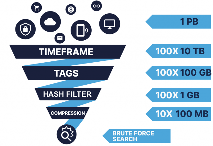 |
Once LogScale has identified the data that needs to be scanned and then identified the events that match that information, LogScale moves on to the more detailed processing of the event data, where LogScale also allows you to reformat, extract and manipulate information through the LogScale Query Language.
MapReduce Strategy
LogScale search is built around a mapreduce strategy. MapReduce allows data to be scanned across multiple nodes in parallel, and then reduced or summarized to filter out and manipulate the information as it is processed.
Many databases use this approach, and MapReduce is used in big data systems like Google's BigQuery and Hadoop. LogScale does mapreduce on smaller chunks of data (segment blocks) and continuously shows partial results to the user. LogScale will typically also search the newest data first. This ensures that LogScale initially returns data very quickly and returns all of the matching data over time.
In the example below, data is scanned in each segment as part of the mapping process, and then reduced within the node before being merged up at the parent reducer and then returned to the user. This distributes the process of scanning across multiple nodes, but aggregates the data to the user through a single process providing the unified, single, result set.
For every map phase there will be a search state. The state will start out empty and then as events are scanned (mapped), the state is updated. The state from one map phase can then be merged (reduced) with states from other map phases. States will then keep being merged (reduced together) as they get higher and higher up the tree and until there is one resulting state.
Let's look at an example. Imagine we are collecting logs from a fleet of web servers and we want to see how many internal server errors we have (i.e. where the status code equals 500):
#source=webserver.log statuscode=500
| count()
The search and map/reduce process works as follows:
An individual mapper process will handle a segment file. For each block in the segment file, the mapper will ask the hash filter if the block contains events with a statuscode field with value 500. If that is the case, the mapper will open and scan the block.
The state for this search is simple and will contain the number of events that has been found matching the filter.
Each map process will handle a set of segments and count how many events matches the filter. Merging the states together for this query is trivial, just add the numbers.
Let's look at a more complex example in more detail:
#source=webserver.log statuscode >= 500
| groupby(statuscode, function=count())
The state of this search is a dictionary having status code as key and the counted number of events with the status code as value. Across two nodes, each node may have a different set of matching events:
Table: Node 1
| statuscode | count |
|---|---|
| 500 | 110 |
| 501 | 52 |
| 502 | 5 |
| 503 | 2 |
Table: Node 2
| statuscode | count |
|---|---|
| 500 | 50 |
| 501 | 10 |
| 502 | 78 |
| 504 | 20 |
When reducing the two result sets, we have to add up the count for each matching statuscode. If the statuscode does not exist in one set, then we create it anyway. Use only that value. The resulting series of events might look like this:
Table: Combined Results
| statuscode | count |
|---|---|
| 500 | 160 |
| 501 | 62 |
| 502 | 83 |
| 503 | 2 |
| 504 | 20 |
This map/reduce process can be used for any event set, and its distributed nature makes it first and practical when used within a cluster that already has the data distributed. The process is also very scalable, working as well, and as easily, across one node as 100 nodes.
State Sizes and Limits
The state model used by LogScale during searches and the map/reduce process works in most cases and is able to keep the state size - the list of events at each phase - small. This helps to support fast searching by allowing the search to be parallelized effectively.
However, for some searches the state size for each phase grows. An increased state size requires more memory to handle the event data, increased time to transfer over the network, and more processing to merge the event data.
To alleviate this problem and increase the overall search performance for queries, LogScale sets a state size. The default is to keep only the newest 200 events in memory. A size limit also applies which may reduce the number of events if the overall size of the events would consume too much memory.
LogScale also uses an approximation (or sketch) algorithm to help keep the results within the size and computational boundary while retaining performance.
For example, the top() function returns the top 200
entries from the result of a search. Finding the most accessed URLs
would require to keep all the different URLs in the search state and
count the number of occurrences of each. Computationally this would be
expensive. The more unique URLs, the bigger the state.
There are no limits to how big the state can be to solve this problem
precisely. Fortunately, a sketch algorithm exists that can give an
approximate result and is bounded in size. Other functions that use the
same approximation technique include count() and
percentile(). See
Accuracy When Counting Distinct Values for more information on the
approximation accuracy.
The use of these approximation algorithms helps to ensure performance and responsiveness for queries, but also means that queries may return indeterminate results.
If a search creates such a result or the size of the results would be
too large, the user will be notified. For example,
groupBy()on a high cardinality field could result
in potentially millions of groups. LogScale calculates an
approximate size of the state and will not allow it to go over
configured limits.
Query Coordination
When a search is submitted, whether by a user or internally, the query is routed to a query coordinator node. The query coordinator node handles the entire process:
Receiving the query
Parses the query
Looks up the metadata for the query in the Global Database to determine which segment files need to processed
Contacts the storage nodes for stored segments
Contacts digest nodes for the most recent data
The query coordinator coordinates internal requests to all the involved nodes. Once the individual nodes have returned result data, the data will be merged together and the results returned to the user through the MapReduce Strategy.
Partial ResultsLogScale provides partial results to the user, returning information even though the search may not have completed. This enables users to see some results almost instantly and be able to iterate and explore the data, particularly through the UI.
To achieve this, the query coordinator manages the way in which it polls nodes for newer results. The metadata returned during the search process by each node provides an indication of when the query can be polled again for new data. You can see this when using a polling query through search API (see Polling a Query Job). The JSON returned by LogScale contains a field, pollAfter that gives an indication of when the client should next poll for new data.
This approach serves two purposes, it provides data to the client quicker, but it also protects nodes from being polled too frequently which would increase load and slow down overall performance. In practice, this means that a new query may have a short poll period (as new data may be available sooner), with the poll time increasing as the result set reaches a more final state.
Searches in the UI
The UI supports all forms of searching, and the time span is set via the UI to allow searching across defined and relative timespans.
When viewing dashboards, LogScale will optimize query executions as much as possible. Similar queries or queries that make use of saved searches will optimize the execution of the query and make use of cached query results when possible.
As a further optimization, LogScale will avoid executing queries (including dashboards) if a browser tab is in the background, or if a widget on an individual dashboard is not currently displayed on screen.
Live Searches
An important feature of LogScale is the ability to search data in real-time. The ingest flow (see Ingesting Data) will process incoming events and make them available for searching in less than a second.
Many queries in LogScale are based on the most recent data, for example:
Show me the response time for user-requests for the last hour
Show the exceptions happening in the application for the last hour
How much money did the web shop make over during the last week?
How many users signed up in the last 10 minutes?
Often these types of searches are used in dashboards or alert searches that are continuously running in the system. It is important that matching events are returned as quickly as possible, but also that they are executed as efficiently as possible since the live queries will always be executing.
To support these live searches, the ingestion pipeline must be efficient enough to avoid delaying data ingestion. The system also needs to efficiently search the new data as soon as it is ingested.
Considering other databases that have to handle this approach generally fall into two groups:
Typical databases may use an approach that regularly polls data that has already been ingested, effectively waiting until the data has been stored to execute a query and return the matching data. Repeated queries at set intervals increase the load on the system. If the data is not organized and indexed temporally then returning the most recent events can also be an expensive operation. The result is that queries only return data after the information has been stored and indexed.
Streaming systems take the opposite approach, searching data as it comes into the system. However, streaming systems are not designed to query historical information; once the data has been processed through the input stream, often the data is discarded.
LogScale combines these two approaches, querying data during the ingestion process while combining that with already ingested historical data. Queries use the same query language for both searches, and LogScale uses the MapReduce Strategy to combine the results as a unified result set.
The figure below shows how the live query process operates:
When starting a live query:
Query coordinator submits the live query to every digest node in the cluster
Each digest node creates a live query processor to execute the query
As events are read from the ingest queue, the events are sent to two locations:
Digest queue for storage
To all live queries that match the tags for the events
Each live query starts with an 'empty' state
As new events are processed and match, they are mapped to create the streaming event set
The digest nodes process both the streaming portion and the historical search. The events from both parts are then merged together to produce the live result set through the standard map/reduce process.
Eventually, the historical search will complete and only the streaming parts will continue collecting new data. It is worth noting that digest nodes will both run a historical part, searching through segment files as well as a streaming part for a given query.
Live Search Operation
Due to the nature of the live search, there are some limits and restrictions on the types of search that can be performed. A live search:
May be terminated without warning
May be impacted by the configuration which sets the limits by which live query jobs are terminated. For self-hosted deployments, see
LIVEQUERY_CANCEL_COST_PERCENTAGEandLIVEQUERY_CANCEL_TRIGGER_DELAY_MS.
Live Search Window
A big challenge for live searches is that data must be removed when it is outside of the request time interval. Aging out data does not naturally fit into the map reduce strategy where all states are merged together. To support aging out data, live searches split the data into buckets:
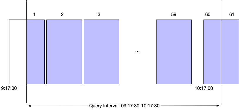 |
By dividing a search into buckets, the last bucket can be dropped when it ages out. New buckets can be added as time moves forward. New events will typically go into the current (rightmost bucket), but delayed events can also land in other buckets matching their timestamp. Each bucket will have its own state so a live search will have multiple states across the range of data.
To create a partial result, the states for the buckets in the current time interval are merged/reduced together into one state to return a result. The length of each bucket determines the precision of the result, since only a whole bucket can be aged out. The important tradeoff being that many buckets requires keeping many states in memory.
The challenge with live searches is, therefore, the potential memory usage. Creating a search using query functions that require large state sizes creates large states for each bucket. To alleviate this, LogScale creates the same constant number of buckets for all live queries.
Efficiency wise, live queries are CPU efficient as they use data stored in the cache after it has recently been processed as part of the ingest flow. This does not eliminate the possibility of creating an expensive live query. Queries with complex regular expressions for example can require a larger amount of processing. Unfortunately, complex live queries can create live queries that are unable to keep up with the events being ingested.
LogScale will automatically kill live queries if they are too expensive. Ingest and digest is prioritized over live search performance.
Live searches are kept alive by LogScale for a long time, even when no clients are polling them. Dashboards are often made up of live searches. If one user has opened a dashboard (and moved on) the live queries will be kept alive and running on the server, so that if a user opens the same dashboard a little later, all the search results will be immediately available.
Live searches will only be kept alive if they completed their historical part of the search. Users can also share the same live searches. If multiple users are looking at the same dashboard they will share the same searches. If one user shares a live search with another user, they will also share the search and see immediate results if the search has been kept alive in the cluster.