
Used with timeChart() or
bucket(), computes the aggregate for one or more
fields over a sliding window of data. This function can only be used as
the function argument with timeChart() or
bucket(). If used elsewhere, an error is reported to
the user.
| Parameter | Type | Required | Default | Description |
|---|---|---|---|---|
buckets | integer | optional[a] | Defines the number of buckets in the sliding time window i.e., the number of buckets in the surrounding timeChart() or bucket() to use for the running window aggregate. Exactly one of span and buckets should be defined. | |
function[b] | Array of Aggregate Functions | optional[a] | count(as=_count) | Specifies which aggregate functions to perform on each window. |
span | long | optional[a] | Defines the width of the sliding time window. This value is rounded to the nearest multiple of time buckets of the surrounding timeChart() or bucket(). The time span is defined as a Relative Time Syntax like 1 hour or 3 weeks. If the query's time interval is less than the span of the window, no window result is computed. Exactly one of span and buckets should be defined. | |
[a] Optional parameters use their default value unless explicitly set | ||||
Omitted Argument NamesThe argument name for
functioncan be omitted; the following forms of this function are equivalent:logscalewindow("count(as=_count)")and:
logscalewindow(function="count(as=_count)")
The window() computes the running aggregate (e.g.
avg() or sum()) for the given
incoming events. For each window, the window() takes
the buckets parameter and uses
this to calculate the rolling aggregate across that number of buckets in
the input.
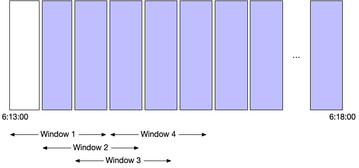
For example, this query calculates the rolling average over the preceding three buckets in the humio for allocBytes:
timechart(span=15s,function=window(function=avg(allocBytes), buckets=3))
|formatTime(field=_bucket,format="%T",as=fmttime)
Tip
Use the Data tab in Time
Chart to view the raw data being used for the chart.
| _bucket | _avg | fmttime |
|---|---|---|
| 1711520025000 | 18410.014084507042 | 06:13:45 |
| 1711520040000 | 23895.214188267393 | 06:14:00 |
| 1711520055000 | 24428.83897158322 | 06:14:15 |
| 1711520070000 | 24178.220994475138 | 06:14:30 |
| 1711520085000 | 24718.239339752407 | 06:14:45 |
| 1711520100000 | 18554.22950819672 | 06:15:00 |
| 1711520115000 | 25638.98775510204 | 06:15:15 |
| 1711520130000 | 18482.970792767734 | 06:15:30 |
| 1711520145000 | 25925.13892709766 | 06:15:45 |
| 1711520160000 | 19303.472527472528 | 06:16:00 |
| 1711520175000 | 25806.04081632653 | 06:16:15 |
| 1711520190000 | 17668.755244755244 | 06:16:30 |
| 1711520205000 | 24431.551299589602 | 06:16:45 |
| 1711520220000 | 17237.956043956045 | 06:17:00 |
| 1711520235000 | 23476.795669824085 | 06:17:15 |
| 1711520250000 | 15585.57082748948 | 06:17:30 |
| 1711520265000 | 22664.589358799454 | 06:17:45 |
| 1711520280000 | 16099.04132231405 | 06:18:00 |
A graphical representation, showing the span of each computed window is shown below.
 |
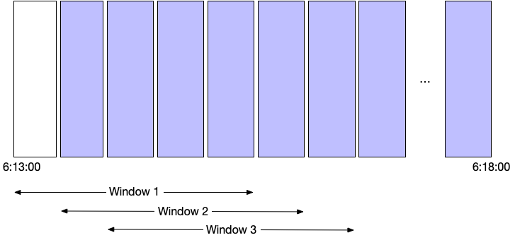
By comparison this query computes the value over the preceding 5 buckets:
timechart(span=15s,function=window(function=avg(allocBytes), buckets=3))
|formatTime(field=_bucket,format="%T",as=fmttime)
The computed average is different because a different series of values in different buckets is being used to compute the value:
| _bucket | _avg | fmttime |
|---|---|---|
| 1711520025000 | 17772.622950819674 | 06:13:45 |
| 1711520040000 | 21970.357963875205 | 06:14:00 |
| 1711520055000 | 22170.04451772465 | 06:14:15 |
| 1711520070000 | 22505.86600496278 | 06:14:30 |
| 1711520085000 | 23378.47308319739 | 06:14:45 |
| 1711520100000 | 23568.354098360654 | 06:15:00 |
| 1711520115000 | 23566.52023121387 | 06:15:15 |
| 1711520130000 | 19816.212271973465 | 06:15:30 |
| 1711520145000 | 24608.287816843826 | 06:15:45 |
| 1711520160000 | 20315.036303630364 | 06:16:00 |
| 1711520175000 | 24221.750206782464 | 06:16:15 |
| 1711520190000 | 19854.064837905236 | 06:16:30 |
| 1711520205000 | 23849.69934640523 | 06:16:45 |
| 1711520220000 | 18996.489256198347 | 06:17:00 |
| 1711520235000 | 22389.50906095552 | 06:17:15 |
| 1711520250000 | 17751.334442595675 | 06:17:30 |
| 1711520265000 | 21959.068403908794 | 06:17:45 |
| 1711520280000 | 17377.422663358146 | 06:18:00 |
This can be represented graphically like this:
 |
If the number of buckets required by the sliding window to compute its
aggregate result is higher than the number of buckets provided by the
surrounding timeChart() or
bucket() function, then the
window() function will yield an empty result.
Any aggregate function can be used to compute sliding window data.
An example use case would be to find outliers, comparing a running average +/- running standard deviations to the concrete min/max values. This can be obtained by computing like this, which graphs the max value vs the limit value computed as average plus two standard deviations over the previous 15 minutes.
| timeChart(function=[max(m1),window([stdDev(m1),avg(m1)], span=15min)])
| groupBy(_bucket, function={ limit := _avg+2*_stddev
| table([_max, limit]) })
window() Examples
Chart 30 minutes running average of cpu load. The time interval of the query must be larger than the window span to produce any result.
timeChart(host, function=window( function=avg(cpu_load), span=30min ))Chart 30 minutes running average and maximum of cpu load. This example specifies three buckets of the outer timechart (each of 10 minutes).
timeChart(host, function=window( function=[avg(cpu_load), max(cpu_load)], buckets=3 ), span=10m)